By Maria Helmrich
At L-IFT, we are in the process of developing a data collection app; a type of platform where our respondents can self-report their data and get access to their results directly.
Having tested the app numerous times, inputting respondents’ data, test building profiles, it repeatedly occurs to me how different everyone is and how every single respondent has a different situation and story to tell. In fact, while in theory of course an average exists, I am tempted to say that there is no such thing as an average respondent; even the respondent who is the average one, very clearly is not representative of the whole group.
There are two stories to tell; we can look at the average at the group level and at the individual level.
Let’s focus first on the group level.
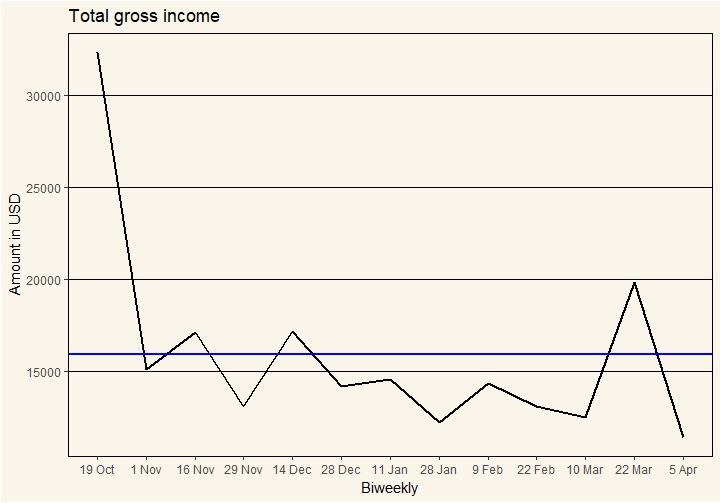
Figure 1: total gross income, n = 570
The above graph shows total gross income amounts in USD for the whole research sample over a six-month research period. This sample consists of 570 respondents from the Financial and Energy Diaries Uganda (FEDU) study, that L-IFT carried out in 2016/2017 in twelve districts of Uganda.The blue horizontal line represents the group average, $15,933. This means that on average, the sum total income of all 570 respondents is $15,933 per biweekly. If we look at the graph, we see that in only four out of the 13 biweeklies, that is only a third of the time, is total income actually above the average. This means that for two thirds of the time, total gross income is actually lower than the average. If we were to take the average amount as a benchmark and assume this to be the amount to base decisions on, we would get disappointing results for total income whereas people would probably expect to be below average half of the time.
While we often look for solutions at the group level, we also need to consider that this group is made up of many individuals who all have their own story and often very different from one another.
Let’s now look at two examples.
On one extreme is one of the lower earners, #112. This is a woman aged 34 who lives in a rural area. Let’s call her Sarah. Sarah’s main activity is farming for own consumption. Her average gross income is $3.24 per biweekly. Looking at the graph, we can see that about half the time (six out of 13 biweeklies) this respondent has a higher income than average, while for the remaining seven, her total gross income is below the average. In fact, for three biweeklies, Sarah earns $0. The highest income occurs in mid-December, $8.57.
The only other income this respondent mentioned is receiving gifts from church, aid, family or inheritance in the first biweekly and 7th (mid-January). She had not reported any savings; neither did she take any loans.
This is an extreme example but there are other similar cases. We can see that her income is unsteady; it is not always clear when it will be a positive or negative value, which makes planning for the future difficult. This respondent will have very different needs from the group as a whole due to her fluctuating and unpredictable income. When looking at the group averages you would not realize easily that these cases exist, because the average covers up the details.

Let’s take another example. One of the higher earners we have is respondent #481. We’ll call him John. John is aged 49 and living in an urban area. On average, per biweekly he earns $524 gross, making him a big contributor to the total group amounts.
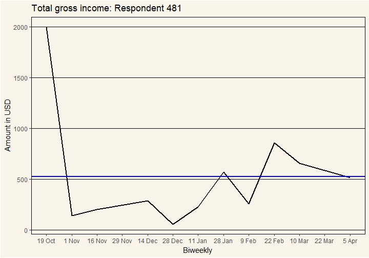
This second respondent shows us another extreme example, but very different from Sarah. However, what we can see in this example (as well as at the group level) is that actually for more than half biweeklies, gross income is less than the average value. This means that on the whole the fluctuations up are higher than the fluctuations down, or to visualize there are a few sharp spikes in many people’s income.
For John, like for the group as a whole, using the average as an indicator would result in too high expectations most of the time, as the majority of times the values are lower than average. This would likely lead to disappointments in the majority of the times.
Another similarity across respondents (and the group) is that income is quite volatile and unpredictable. Some weeks there might be a lot of incoming money while others there might be none at all. This is a lesson for financial service providers who might, for example, adapt their repayment schedules to be more flexible to accommodate the fluctuating income of their clients.
This insight into the income patterns and income distribution across the entire group is one of the valuable aspects of diaries research; getting such in-depth information on every respondent that you are really able to form a story about each person is beneficial and raises the awareness of the wide range of patterns across different individuals. The wealth of information diaries provide, is able to compliment other information. Quoting from the US Financial Diaries, “the intensive nature of the Diaries mean[s] that forming a nationally representative sample [is] impossible. Instead, we aim for the richest, most complete stories we [can] glean from a select group of households.” Indeed, this is another lesson to learn from above; getting detailed individual data to form their comprehensive stories, while taking care to not generalize for the group.